Difference between revisions of "FractBias"

Revision as of 13:53, 14 October 2015

Background

Whole genome duplications (WGDs) and genome fractionation are covered more thoroughly in other CoGepedia entries. In short, WGDs create two or more copies of a genome: which are referred to as subgenomes. The duplicate subgenomes then undergo gene loss in a process called fractionation which is part of returning to a diploid state, diploidization. All things being equal, one may assume that fractionation would occur randomly across the redundant genes created after a WGD, however bias towards gene loss on one genome, called fractionation bias, has been observed in several species including: maize ^[1], Brassica rapa ^[2], and rainbow trout ^[3].

Overview

Figure 1. A demonstration of which genes are included in the FractBias analysis of retained genes when the include "All genes" setting is selected. All genes that exist on target genome chromosomes will be used to determine the sliding window size and calculate the number of retained genes on query chromosomes.

Figure 2. A demonstration of which genes are included in the FractBias analysis of retained genes when the include "Only retained genes" is selected. Genes unique to either the target or to the query genome will not be considered in either the window size or in calculating the number of retained genes within in the window.

What goes in

1. Two assembled genomes that have annotated coding sequences (CDS)
2. A syntenic ratio set by the user (identified by empiric tests outside of the FractBias tool)
   1. The genome with a lower ratio will be the target genome
   2. The genome with a higher ratio will be the query genome
3. The full GFF of the target genome
4. The syntenic blocks identified by SynMap
5. Setting defined by the user
   1. What genes should be counted
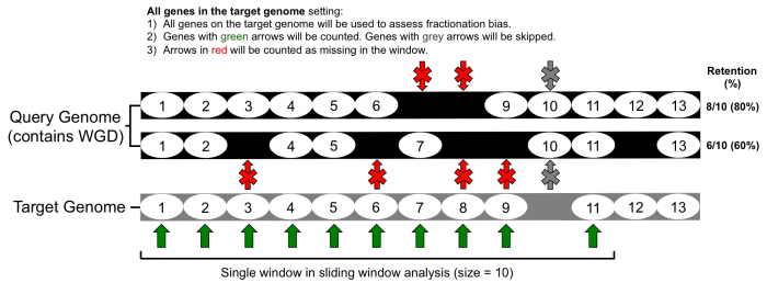
      1. Count all genes present on the target genome (refer to Figure 1)
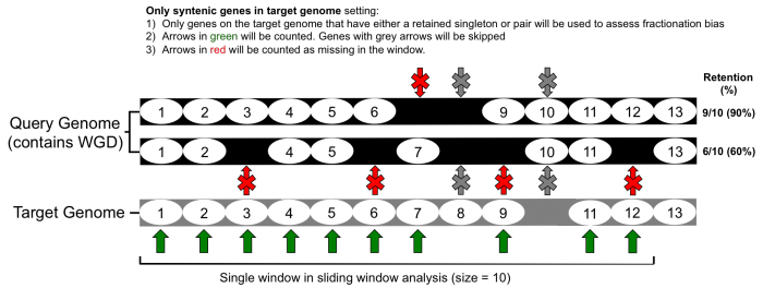
      2. Only count genes that are retained in both genomes (refer to Figure 2)
   2. Target chromosome number
   3. Query chromosome number
   4. Window size

What comes out

1. A figure containing a subplot for every target genome chromosome
2. Links to the raw data used to create the subplots

FractBias Methods

FractBias is a tool used to assess fractionation bias after whole genome duplications (WGDs). To investigate fractionation bias, select an organism that has experienced a WGD (e.g. maize) which will become the 'query' genome, and an organism that diverged before the WGD (e.g. sorghum recently diverged before the WGD in maize). The following is a list of all user inputs:

User Input

1. Select two genomes to compare in the SynMap tool.
2. Select the SynMap 'Syntenic Depth' option under 'Analysis Options.'
3. Set syntenic depth ratio between genomes (determined by empirically outside of this tool).
4. Set how many target genome chromosomes should be included in the analysis. There is a maximum of 40 target chromosomes that can be included, and the longest chromosomes are selected first.
5. Set how many query genome chromosomes should be included in the analysis. There is a maximum of 40 query chromosomes that can be included, and the longest chromosomes are selected first.
6. Set the size of the sliding window during analysis.

FractBias tool analysis

Once all of the user input options are filled and submitted, the FractBias tool then runs an analysis in the following steps:

1. The coordinates for syntenic regions between the genomes are determined by the SynMap tool
2. The syntenic genes are then parsed according to the 'target' and 'query' genomes. The genome with the lower syntenic depth ratio is set as the target genome; the genome with the higher ratio is set as the query genome.
3. A list of genes present on every target genome chromosome is made and ordered according to start site (bp) in the annotation (gff/gtf file).
4. The FractBias tool then goes through the list of each target genome gene, and determines if it has a retained homolog on one (or more) of the query chromosomes.
5. Finally, the FractBias tool runs a sliding window analysis to calculate how many genes are retained for each query chromosome.
6. A figure is generated that contains a subplot for every target genome chromosome
   1. The x-axis: target genome gene order number in sliding window analysis according to order of start site in genome annotation (gff/gtf).
   2. The y-axis: percent of retained genes from the target genome present on each query chromosome within that window.
7. The SynMap raw data, the FractBias data, genes identified using FractBias, and the images can be downloaded through links for further use.

Example Output

Figure 3. A demonstration of how the sliding window analysis is carried out. The window size is set by the user, and begins at the first annotated gene on the target chromosome (x = 1 on the x-axis of the output subplot for that target chromosome). Then the window determines the percentage of homologs that exist on all query genome chromosomes within that window (output as the y value for each query genome chromosome in the output subplot). The window then slides down a single gene, and recalculates the percentage of corresponding homologs on each query genome chromosome (x = 2 and corresponding y values). This repeats until the window reaches the last gene on the target genome chromosome, and then the analysis terminates. Analysis is only carried out on full window sizes; any chromosome or window containing less genes than the user set window size is terminated. Results from this analysis are presented in Table 1 and 2 below.

Figure 4. An example FractBias subplot generated from Table 1 "All Genes Example Data Table."

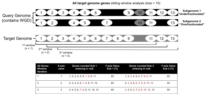
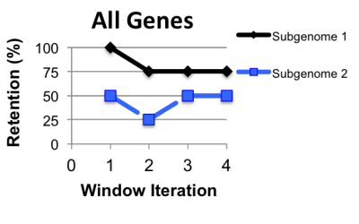
To demonstrate how the FractBias tool works, an example of a single syntenic block with eight genes is presented. The FractBias tool can be run with either "all genes" included, or "only retained genes" included. The "all genes" option will include all the genes from the target genome

'*' Red numbers are counted as zeros in sliding window analysis

Figure 5. An example FractBias subplot generated from Table 2 "Only Retained Genes Example Data Table."

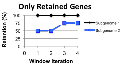
If the include "only retained genes" option is set, all unique genes from either the target or query genome are not considered for the fractionation bias analysis. This option can be used to remove variation from two genomes that have diverged over longer periods and clean up the analysis.

'*' Red numbers are counted as zeros in sliding window analysis

Biological Examples

Sorghum and Maize Fractionation Bias

Arabidopsis and Brassica Fractionation Bias

Esox and Oncorhynchus Fractionation Bias

References

- ↑ Schnable, J.C. et al. Dose–sensitivity, conserved non-coding sequences, and duplicate gene retention through multiple tetraploidies in the grasses. Front. Plant Sci. http://dx.doi.org/10.3389/fpls.2011.00002 (2011)
- ↑ Cheng, F. et al. Biased gene fractionation and dominant gene expression among the subgenomes of Brassica rapa. PLOS ONE DOI: 10.1371/journal.pone.0036442 (2012)
- ↑ Berthelot, C. et al. The rainbow trout genome provides novel insights into evolution after whole-genome duplication in vertebrates. Nature Communications 5: DOI:10.1038/ncomms4657 (2014)